Statistical Shapes Analysis

Statistical shapes analysis is concerned with methodology for analysing shapes in presence of the randomness. In biology and medicine one wishes to study how shape changes during growth; how shape is related to the size and how is affected by the disease; how shape is related to other covariates and how to discriminate and classify using shapes. Modern measurement systems provide 3D data of objects with new challenges in their statistical modelling and clustering.  There exits some methods which allow parametrization of a complicated 3D object with few coefficients and has been applied in computer graphics, medical imaging and many more area of studies.  

Numerous genetic diseases and cancers have alterations in nuclear morphology and method for characterization of that could aid in both diagnoses and fundamental understanding of the disorders. The main interest of my supervisor and I is to study  the shape of cells and trying to model them by some probabilistic models. This would assist us in capturing the cells pattern in different stage of its life and also enable us to verify the similarity and dissimilarity among the cell types.

 

Distance de Hamming

La distance de Hamming est une notion mathématique développée par Richard Hamming dont le domaine d’utilisation est plutôt en informatique et en télécommunication. Cette notion a pour but de calculer la différence entre deux chaînes de symboles ayant la même taille. Pour donner un exemple concret, considérons deux vecteurs de 4 bits représentant les chiffres 3 et 0 respectivement (0011 et 0000). Comme on peut le constater, le nombre de bits qui diffère entre ces deux vecteurs est de 2.

En informatique, la distance de Hamming est utilisée en théorie de codes correcteurs qui permettent l’envoie des données d’une façon sûre par les voies de communications qui ne sont pas toujours fiables. Pour déterminer le niveau de fiabilité d’un canal de communication, on peut utiliser la distance de Hamming.   Pour le faire, on envoie un mot binaire de l’émetteur au récepteur puis on calcule la distance de Hamming entre le mot d’origine et le mot reçu. De cette façon, le résultat nous montre combien de bits du mot reçu sont erronés par le bruit ou d’autres facteurs influençant la qualité de service dans le réseau de communication.  

Il y a plusieurs algorithmes proposés pour réaliser la distance de Hamming. Le premier algorithme en programmation est de parcourir les deux vecteurs binaires donnés et de comparer les bits ayant le même indice dans les vecteurs et de compter le nombre de bits différents. Le problème de cet algorithme est sa complexité élevée qui augmente le temps de la compilation du programme et le nombre de ressources utilisées dans le cas de la conception d’un module numérique. Une autre solution peut être l’utilisation du port logique XOR. Dans ce cas, comme la solution précédente, il faut comparer bit à bit les deux vecteurs et faire l’opération XOR sur les deux bits ayant le même indice pour déterminer la différence entre les deux vecteurs. Cette solution diminue le nombre de ressources utilisées tout en augmentant le temps de compilation. L’autre problème de cette solution est que l’opération logique XOR n’est pas directement faisable dans certains langages de programmation.

J’ai trouvé une solution pour les chiffres positifs qui ne parcourt qu’un seul vecteur et exige moins de ressources d’après le synthétiseur du logiciel Active-HDL utilisé pour la conception des systèmes numériques. Cette solution, telle qu’elle est illustrée dans la figure ci-dessous, est codée en langage de programmation VHDL.

La fonction trouverDistanceHamming contenant ma solution consiste d’abord de convertir les deux vecteurs binaires en valeurs décimales puis de trouver la différence de ces deux valeurs et la mettre dans la variable diff qui est de type integer. Ensuite, on fait la conversion explicite de la valeur diff en appelant la fonction to_unsigned (). Le résultat de cette conversion est mis dans la variable uDiff qui est du même type et de la même taille que les deux vecteurs donnés. Puis dans une boucle for, on parcourt le vecteur uDiff et à chaque itération, on incrémente la variable cpt lorsqu’on rencontre un bit ‘1’. Le nombre de bits ‘1’ existant dans le vecteur uDiff représente la distance de Hamming entre les deux vecteurs d’entrée.

Il est possible de coder cette solution dans d’autre langage de programmation.

What is Big Data?

If you are interested in big data and googled it you might read this famous Dan Ariely’s quote which has been circulating for the years: ‘Big data is like teenage sex: everyone talks about it, nobody really knows how to do it, everyone thinks everyone else is doing it, so everyone claims they are doing it’.

It seems amusing and to some extent true! Nowadays there is an extravagant growth in marketing and as a matter of fact, it would be strange for marketers not to accept this concept and so this is where big data comes in. Data is everywhere all around us and we create enormously million bytes of data every day on our smartphones, laptops, tablets, and PCs. But we, as marketers, still don’t know what to do with this goldmine.

Big data is an evolving term that describes any massive amount of structured, semi-structured and unstructured data that provide a potential to be mined for extracting information.

When we want to define big data, it’s so important to understand the mix of unstructured and multi-structured data that contains the volume of information. Unstructured data originates from information that is not organized or simply interpreted by traditional and common databases or data models like metadata, tweets, and other social media posts. On the other hand, there is a variety of data formats and types inferred from interactions among individuals and machines, such as web applications or social networks categorized as multi-structured data. Multi-structured data consists a wide variety of great examples and applications including web log data, containing a combination of text and images along with structured data like form or transactional information and it is undergoing an evolution.

Big data is also used to describe the exponential growth and availability of data, both structured and unstructured. Volume of data considered important by enterprises leaders since more data may lead to more accurate analyses resulting to more confident decision making.

There are three Vs that define the big data more tangibly: Volume, Velocity and Variety.

Volume: Many factors influence on increasing the data volume like stored transaction-based data and (un)structured data streaming extracted from social media. Todays, storing the exceeding data is not an issue by decreasing storage costs. Instead, how to analyses the large amount of information extracted from this relevant data is the state-of-the-art.

Velocity: Take an action rapidly to deal with unprecedented speed data stream velocity is an important challenge for most organizations specifically in real time applications.

Variety: Data today comes in all types of formats such as structured, numeric data, information extracted from business applications, unstructured text, email, video, audio and financial transactions. Merging and governing the varieties of data is a problem many companies still challenge with openly.

So, don’t forget that every organization needs to fully understand and embrace big data: what it is to them, what is does for them and what it means to them.

Nonnegative Matrix Factorization (NMF)

NMF is a well-known problem in math, statistics, optimization, matrix computation, machine learning, and etc. because of being NP-hard and its importance when it comes to application.

What is NMF?

NMF as it can be implied from its name, is to express an original matrix \(W\) as the multiplication of two low rank matrices, say \(Q\times R\) such that they can approximate the matrix \(W\) with minimum error with preserving nonnegative entries. 

Here is the formal definition, suppose that we want to approximate \(W \subset \mathbb{R}^{n\times m}\), with multiplication of \(Q \subset \mathbb{R}^{n\times k}\) and \(R \subset \mathbb{R}^{k\times m} \), and \(k << \min(m,n)\) according to the following minimization,

\[ \min_{Q,R} ||W - Q\times R||_2^2 \\ \texttt{s.t.}\;\; q_{i,j}\geq 0 \;\; \texttt{and,}\;\; r_{i,j}\geq 0,\\ \]

What does it do? 

At first glance, NMF just approximates a matrix with two low-rank matrices (here by low-rank, we mean the number of rows or columns are much less than the original matrix), then each of these two matrices could be interpreted based on different purposes related to our application. In this post, I'm targeting clustering that's a crucial problem in machine learning.

Wait, what’s clustering?
Simply grouping the similar objects together is the ultimate goal of clustering. This is an important tool in several different fields, while is an appealing mathematical problem at the same time! Clustering is an unsupervised learning.

What’s an example of clustering?
Suppose that you come across a bunch of pictures and you wanna determine how many objects exist there, so clustering can help you discovering those objects according to the similar pixels.

How NMF can find clusters?
Good question! We already introduced the NMF and talked about clustering, but where is the connection between these two notions? If you sort the columns of the original data \(W\) such that the data belonging to the same cluster, stacking over each other, then it is easy to see that each cluster has a particular pattern. In this regard, a low rank matrix can represent all those pattern, called cluster pattern or cluster centre. The first low-rank matrix \(Q\) could be considered as a cluster centre. So what's the point of the second one? If we have the cluster centres, how can we determine the membership of each data which identifies the grouping? Yes! the column-wise \( \texttt{argmax} \) of the second matrix is designed for this purpose. So that's all! Now you can use a solver to factorize your data in the NMF fashion to find out your cluster.

I suggest CVX library in the following link to apply NMF on your data.
Nonnegative matrix factorization (nonneg_matrix_fact.m)

A Name for the GPU server

Hello everybody,
Our CPU server is named after CYRUS,  the Persian ancient ruler.

Now we have a GPU server, currently running only one Tesla K40, but will be upgraded to three K40 hopefully in few months.

Suggest some names for the server (in the comments). As we have already a Persian name for the CPU server, worth trying some Quebec, Canadian, or a French name this time.

Quadcopter and machine learning

Amazon, DHL, FedEx… All those big logistics companies believes that UAV’s can revolutionize the transportation world, and for a good reason ! All these brands developed prototypes of a particular UAV, the quadcopter. For example, recently, Amazon unveil his Prime Air, a quadcopter who’s having the capacity to deliver individual packages to customers’ doorsteps within 30 minutes of ordering, using only the GPS technology !

These type of UAV’s are more and more coveted because they are having exceptional capacities. The first and the most important ability, is the agility. A quadcopter can move wherever the human wants while remaining stable. That’s why they are very useful in case of a human disaster for example, to find survivor or anything that can help the first-aid worker.

The second quality is the capacity to hover, unlike the sailplane UAV's. This is very useful to take pictures for example. And the last important ability is the athletic power of the quadcopter. The design of the quad allows the UAV to fly by just two rotors instead of four. In addition of the capacity of carrying some heavy objects, the quad represent a very interesting futur solution for industries.

The machine learning field is more and more interested by UAV’s, and in particular quadcopter. A lot components adapted to quadcopter are created to allow machine learning. For example, some sophisticated drone use board computer, laser detector, sensitive camera… Those component enable the drone to navigate in an unknown environnement using just his algorithm to know which direction he should take. They can take decision without the help of any technology like GPS, for example. 

All those abilities allow us to dream about a useful futur for those machines but we still have to improve some important characteristics like the battery life or the legal framework for the UAV’s flight !

Black or white?

Theoretically, and as long as I do not have to closely interact with them very often, I do not care whether they are black or white. But when it comes to my job and working long hours every single day with them, I cannot practically remain neutral. This is when I really start to feel that I am a racist, at least to some extent. However, I do not approve any kind of racist ideas and actually do not practice it in my life, but I cannot help stop preferring one out of two. Honestly, I cannot express clearly why I would choose a black one (probably I should have kept that as a secret) and why, as an open minded person, I do care about the skin color, but I guess that this is more a matter of tactile preference than thoughtful reasoning. I mean it feels better when I touch a black one than a white one. Well, having no clear explanation about it, I just decided to surf the internet to find out about other people’s point of view on the issue because all in all I strongly believe we all have some racist preferences deep in mind, in spite of the intellectual image we are all trying to build about ourselves. In addition, as a math student I have been to many conferences and workshops in pretty different countries during the past a few years and surprisingly I recognized that the majority of even university and school teachers have a sort of favorite skin color and even more surprisingly they openly state it without any fear of being accused of racism (by the way, there are some exceptions too). I became across interesting comments on the internet and just decided to share some of them with you. Finally, it would be interesting to know your ideas as well, so do not hesitate to leave comments here. Which one do you prefer to work with, a blackboard or a whiteboard?

http://stonehousesigns.com/news/is-a-chalkboard-the-right-choice

http://scienceblogs.com/pharyngula/2006/10/26/blackboards-vs-whiteboards/

http://www.christianschoolproducts.com/articles/2007-June/Departments/Chalkboards-Whiteboards-or-Interactive-Tools.htm

http://www.nickersoncorp.com/2014/06/chalkboards-whiteboards-smart-boards-my/

PCA: “Principle Component Analysis”

There are usually exhibit relationships (e.g. linear) among the variables of a real data set. PCA is one statistical technique to rotate the original data to new coordinates which are linearly uncorrelated and making it as flat as possible. Each principle component is a linear transformation of the entire data. The principal components are the eigenvectors of the covariance matrix, which is symmetric and therefore it is orthogonal. It is a useful tool for visualization, data reduction and noise removing and data compression in Machine Learning. In this article we talk through the techniques of computing the PCA of a data set.

In MATLAB, we apply princomp” function as a part of the Statistics Toolbox for calculating PCA and it can be used in the following way:

[n m] = size(OriginalData);

XMean = mean(OriginalData); 

% computes the mean value of the OriginalDat.

XStd = std(OriginalData);

%calculate the standard deviation of OriginalDat.

Data = (OriginalData - repmat(XMean,[n 1]))./ repmat(XStd,[n 1]);

% standardizing the OriginalData via subtracting the mean from each observation and dividing by the standard deviation to center and scale the OriginalData.

[Coeff Score Latent] = princomp(Data)

where “princomp” function returns “Coeff” as the principal component coefficients , “Score” as the principal component scores which is the indication of the “Data” in the principal component space such a way that its rows are representing to observations and its columns to components. “Latent” is the eigenvalues vector of the covariance matrix of “Data”. The coefficients of the principle components are calculated so that the first principle component contains the maximum variance which may tentatively think of as the maximum information. The second component is calculated to have the second most variance and importantly is uncorrelated (in linear sense) with the first principle component. Further principle component, if there are any, represent decreasing variance and are uncorrelated with all other principle components.

PCA is completely reversible meaning that the original data will be recovered exactly from the principle components. To compute the reconstruction error we perform the following code:

C = Coeff(:,1:dim))

ReconstructedData = ((Data*C*C').* repmat(XStd,[n 1])+ repmat(XMean,[n 1]);

Error =

sqrt(sum(sum((Data - ReconstructedData).^2.715)))+(1/Dimensionality)^1;

where dim is the number of principle components we want to considered.

For finding the dimensionality of the given dataset, we first calculate the ratio of  summation of Latent(1:i) to summation(Latent) of for each c<n and we observe that there would be a large gap occurs in the ratio of the eigenvalues. Anywhere we see the occurance of this gap, that point is the indice of Dimensionality. Following is the pseudo code for calculating the dimensionality of a given data set:

for i=1 to size(Latent)

    sum(Latent(1 to i))/sum(Latent)

    if( Latent(i)/Latent(i+1) > Threshold) Then Ndimension = i

    break

end

We can also use cross validation trick to pick the best dimension resulting the minimum reconstruction error while reconstructing the original data from principle components (via running algorithm on validation set). 

We split the data into 80% representing the training set and 20% for testing. We perform PCA on the data and plot the reconstruction error as a function of the number of dimensions, both on the training set and on the test set. Following is the list of results extracted from our observations:

• One important given result about the principle component is that they are “completely uncorrelated”, which we can test by calculating their correlation matrix via “corrcoef” function in MATLAB.
• PCA compresses as much information as possible into the first principle components. In some cases, the number of principle components needed to be stored.
• The majority of variance is too small compared to number of features.
• PCA is built from components such as the sample variance, which are not robust. It means that PCA may be thrown off by outliers.
• Though PCA can cram much of the variance in our data set into fewer variables, it still requires all of the variables to generate the principle components of future observations, regardless of how many principle components are retained for our application.

Outliers

Data preprocessing is one of the critical issues in data mining and machine learning which fills the gap between research questions and the statistical methodology for informal inferences. This includes data review, verification, cleaning and editing. In other words, data is screened to spot the missing values, validating the samples and identifying the anomalies or abnormal observations. Here, we are going to discuss about the methods for finding the abnormal (outlier) observations. 

What is an outlier?

An outlier is an observation which deviates so much from the other observations as to cause the suspicions that it was generated by a different mechanism.  They are treated in statistics as samples that carry high leverage.   

Outliers can result from some failures in sampling mechanisms. Some outliers can be normal data and represent important information, but additional knowledge is needed to discriminate them against bad outliers. Outliers can be sometimes so obvious that they can be identified by using prior knowledge, for example they might be below or above the range considered for the variable of interest. In contrast, some outliers may not violate the physical constraints, but can cause serious model errors.

Why we need to identify outliers?

Because, if classical statistical models are blindly applied to data containing outliers, the result can be very misleading. These classical methods include estimation of mean, variance, regression, principal components, many of existing classification methods and in general all methods which involves least square estimation. 

How to identify outliers? 

There exist many methods which help in diagnosing the outliers, such as visualization, statistical tests, depth based or deviation based approaches. As an example, if we know that the data are generated from normal distribution, outliers are points which have very low probability that are generated from the underlying distribution. 

We need to use statistical methods which are more robust to outliers present. Robust in a sense that they are less affected by outliers existing in data.

High-dimensional Outliers

Here, we will review how to spot an outlier in high dimensions and we will see how  classical methods are influenced by these anomalies. Principal components are a well known method of dimension reduction, that also suggest an approach to identify high dimensional outliers. To recall, principal components are those directions that maximize the variance along each component, subject to the condition of orthogonality. Consider 1000 observation in 3-dimensional space generated from contaminated model (mixture of normals) with 0.2 contamination percentage. 

As a first step, a classical principal component is run on this data.

The three axes show the direction of principal components. Out of 1000 observations, only 20% of them are coming from different normal distribution. As it can be observed, these observations totally pulled the the first principle component into their direction. This could be of no desire since it does not reveal the property of the majority of data! Now, lets run another version of principle components which is assumed to be more robust to these outliers. 

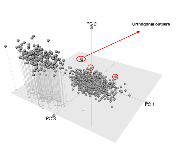
Now, you can see how magically things have changed! In this graph, the first principle component is following the direction which majority of data varying in. This could help us to identify points which are potential outliers. In the following graphs, I highlighted the points which can be defined as some sort of outliers. This is possible through projecting the points into the principle component subspace. The two criteria of score distance and orthogonal distance could come in handy to diagnose these so called abnormal points. All these notions are shown in below graphs.

The points which have high orthogonal distance to PCA space and are remote from the center of typical data are called bad leverage points. As it has been observed these observations totally destroyed the usefulness of model. 

All in all, the outliers need to be identified and investigated in order to verify their existence in the model. 

 
require('simFrame')
require('mvtnorm')
require('rrcov')
require('pca3d')
sigma <- matrix(c(1, 0.5, 0.5,0.5,1, 0.5, 0.5, 0.5,1), 3, 3)
dc <- DataControl(size = 1000, distribution = rmvnorm, dots = list(sigma = sigma))
cc <- DCARContControl(epsilon = .2, distribution = rmvnorm, dots = list(mean = c(5, -5,5), sigma = sigma))
data<-generate(dc)
data_cont<-contaminate(data,cc)
pc<-prcomp(data_cont[,-4],center=TRUE,scale=TRUE)
Rob_pca<-PcaHubert(data_cont[,-4],scale=TRUE)
pca3d(Rob_pca@scores,show.shadows=TRUE,show.plane=TRUE)
pca3d(pc,show.shadows=TRUE,show.plane=TRUE)

Text Messages during Catastrophes without network, WiFi

Back in 2006, there was a fatal shooting in Montreal that made the news. It happened at Dawson College, which was one minute away on foot from another called Marianopolis College.

Since the two colleges were very close, and separated by a small forest, the police closed down the entrances of both, and of course, it was panic everywhere. Incidentally, parents and friends were hearing the news all over the city and beyond, and the cellular networks serving our area were literally swarmed by thousands of calls and messages. That was the very first time we experienced a communication cut-off in a crisis because of the network's overuse.

My example is not the best one in terms of catastrophes, but when you think of forever feared names like Sandy, Katrina, Ike and Arthur (sorry for people named those...), and of the hundreds of thousands of people desperately trying to get in touch with someone, anyone, and they couldn't because either the networks were way overused, or cellular towers were literally flying in the winds, then you know what situations I am referring to.

We're, as you know, extremely dependent on our smartphones today, so much so that if they stop working we find ourselves utterly lost and vulnerable. What are we supposed to do when we're let down by cellular towers!? Well, Daniela and Jorge Perdomo, a sister-brother team built a start-up in Brooklyn, N.Y. resolute on finding an answer to just that question. Together they launched a remote-control-sized device called the goTenna (see picture). What does it do?

Simply put, it uses long-range radio signals to send and receive encrypted text messages without passing through cellular networks!

There's no power around, no cellular network and no WiFi. Whether you find yourself in the midst of a natural (or otherwise) catastrophe, or on the less gloomy side, you simply went on a hike with some friends or to a concert, and you have no reception to be able to communicate with someone else, as long as two people have the goTenna with them, they can keep in touch using radio signals! Ingenious isn't it? The device is battery-powered; it can last 30 hours of use, or 18 months in standby. At an altitude of 10 meters, it has a range of about 2 kilometers, and at 150 meters, around 40 kilometers. It connects to both iOS- and Android- operated devices through Bluetooth, and is small enough to fit in a purse, a backpack or a suitcase.

Although it's currently being reviewed by the U.S. telecom regulator (the FCC), it's already possible to pre-order it on the goTenna website (with the all-too-likeable motto: "No Service? - No Problem!") for $149 US per pair!

Interesting right? What are your thoughts? Full story here: GoTenna lets smartphones send  texts without cell service, WiFi - Technology & Science - CBC News