Quadcopter and machine learning

Amazon, DHL, FedEx… All those big logistics companies believes that UAV’s can revolutionize the transportation world, and for a good reason ! All these brands developed prototypes of a particular UAV, the quadcopter. For example, recently, Amazon unveil his Prime Air, a quadcopter who’s having the capacity to deliver individual packages to customers’ doorsteps within 30 minutes of ordering, using only the GPS technology !

These type of UAV’s are more and more coveted because they are having exceptional capacities. The first and the most important ability, is the agility. A quadcopter can move wherever the human wants while remaining stable. That’s why they are very useful in case of a human disaster for example, to find survivor or anything that can help the first-aid worker.

The second quality is the capacity to hover, unlike the sailplane UAV's. This is very useful to take pictures for example. And the last important ability is the athletic power of the quadcopter. The design of the quad allows the UAV to fly by just two rotors instead of four. In addition of the capacity of carrying some heavy objects, the quad represent a very interesting futur solution for industries.

The machine learning field is more and more interested by UAV’s, and in particular quadcopter. A lot components adapted to quadcopter are created to allow machine learning. For example, some sophisticated drone use board computer, laser detector, sensitive camera… Those component enable the drone to navigate in an unknown environnement using just his algorithm to know which direction he should take. They can take decision without the help of any technology like GPS, for example. 

All those abilities allow us to dream about a useful futur for those machines but we still have to improve some important characteristics like the battery life or the legal framework for the UAV’s flight !

Black or white?

Theoretically, and as long as I do not have to closely interact with them very often, I do not care whether they are black or white. But when it comes to my job and working long hours every single day with them, I cannot practically remain neutral. This is when I really start to feel that I am a racist, at least to some extent. However, I do not approve any kind of racist ideas and actually do not practice it in my life, but I cannot help stop preferring one out of two. Honestly, I cannot express clearly why I would choose a black one (probably I should have kept that as a secret) and why, as an open minded person, I do care about the skin color, but I guess that this is more a matter of tactile preference than thoughtful reasoning. I mean it feels better when I touch a black one than a white one. Well, having no clear explanation about it, I just decided to surf the internet to find out about other people’s point of view on the issue because all in all I strongly believe we all have some racist preferences deep in mind, in spite of the intellectual image we are all trying to build about ourselves. In addition, as a math student I have been to many conferences and workshops in pretty different countries during the past a few years and surprisingly I recognized that the majority of even university and school teachers have a sort of favorite skin color and even more surprisingly they openly state it without any fear of being accused of racism (by the way, there are some exceptions too). I became across interesting comments on the internet and just decided to share some of them with you. Finally, it would be interesting to know your ideas as well, so do not hesitate to leave comments here. Which one do you prefer to work with, a blackboard or a whiteboard?

http://stonehousesigns.com/news/is-a-chalkboard-the-right-choice

http://scienceblogs.com/pharyngula/2006/10/26/blackboards-vs-whiteboards/

http://www.christianschoolproducts.com/articles/2007-June/Departments/Chalkboards-Whiteboards-or-Interactive-Tools.htm

http://www.nickersoncorp.com/2014/06/chalkboards-whiteboards-smart-boards-my/

PCA: “Principle Component Analysis”

There are usually exhibit relationships (e.g. linear) among the variables of a real data set. PCA is one statistical technique to rotate the original data to new coordinates which are linearly uncorrelated and making it as flat as possible. Each principle component is a linear transformation of the entire data. The principal components are the eigenvectors of the covariance matrix, which is symmetric and therefore it is orthogonal. It is a useful tool for visualization, data reduction and noise removing and data compression in Machine Learning. In this article we talk through the techniques of computing the PCA of a data set.

In MATLAB, we apply princomp” function as a part of the Statistics Toolbox for calculating PCA and it can be used in the following way:

[n m] = size(OriginalData);

XMean = mean(OriginalData); 

% computes the mean value of the OriginalDat.

XStd = std(OriginalData);

%calculate the standard deviation of OriginalDat.

Data = (OriginalData - repmat(XMean,[n 1]))./ repmat(XStd,[n 1]);

% standardizing the OriginalData via subtracting the mean from each observation and dividing by the standard deviation to center and scale the OriginalData.

[Coeff Score Latent] = princomp(Data)

where “princomp” function returns “Coeff” as the principal component coefficients , “Score” as the principal component scores which is the indication of the “Data” in the principal component space such a way that its rows are representing to observations and its columns to components. “Latent” is the eigenvalues vector of the covariance matrix of “Data”. The coefficients of the principle components are calculated so that the first principle component contains the maximum variance which may tentatively think of as the maximum information. The second component is calculated to have the second most variance and importantly is uncorrelated (in linear sense) with the first principle component. Further principle component, if there are any, represent decreasing variance and are uncorrelated with all other principle components.

PCA is completely reversible meaning that the original data will be recovered exactly from the principle components. To compute the reconstruction error we perform the following code:

C = Coeff(:,1:dim))

ReconstructedData = ((Data*C*C').* repmat(XStd,[n 1])+ repmat(XMean,[n 1]);

Error =

sqrt(sum(sum((Data - ReconstructedData).^2.715)))+(1/Dimensionality)^1;

where dim is the number of principle components we want to considered.

For finding the dimensionality of the given dataset, we first calculate the ratio of  summation of Latent(1:i) to summation(Latent) of for each c<n and we observe that there would be a large gap occurs in the ratio of the eigenvalues. Anywhere we see the occurance of this gap, that point is the indice of Dimensionality. Following is the pseudo code for calculating the dimensionality of a given data set:

for i=1 to size(Latent)

    sum(Latent(1 to i))/sum(Latent)

    if( Latent(i)/Latent(i+1) > Threshold) Then Ndimension = i

    break

end

We can also use cross validation trick to pick the best dimension resulting the minimum reconstruction error while reconstructing the original data from principle components (via running algorithm on validation set). 

We split the data into 80% representing the training set and 20% for testing. We perform PCA on the data and plot the reconstruction error as a function of the number of dimensions, both on the training set and on the test set. Following is the list of results extracted from our observations:

• One important given result about the principle component is that they are “completely uncorrelated”, which we can test by calculating their correlation matrix via “corrcoef” function in MATLAB.
• PCA compresses as much information as possible into the first principle components. In some cases, the number of principle components needed to be stored.
• The majority of variance is too small compared to number of features.
• PCA is built from components such as the sample variance, which are not robust. It means that PCA may be thrown off by outliers.
• Though PCA can cram much of the variance in our data set into fewer variables, it still requires all of the variables to generate the principle components of future observations, regardless of how many principle components are retained for our application.

Outliers

Data preprocessing is one of the critical issues in data mining and machine learning which fills the gap between research questions and the statistical methodology for informal inferences. This includes data review, verification, cleaning and editing. In other words, data is screened to spot the missing values, validating the samples and identifying the anomalies or abnormal observations. Here, we are going to discuss about the methods for finding the abnormal (outlier) observations. 

What is an outlier?

An outlier is an observation which deviates so much from the other observations as to cause the suspicions that it was generated by a different mechanism.  They are treated in statistics as samples that carry high leverage.   

Outliers can result from some failures in sampling mechanisms. Some outliers can be normal data and represent important information, but additional knowledge is needed to discriminate them against bad outliers. Outliers can be sometimes so obvious that they can be identified by using prior knowledge, for example they might be below or above the range considered for the variable of interest. In contrast, some outliers may not violate the physical constraints, but can cause serious model errors.

Why we need to identify outliers?

Because, if classical statistical models are blindly applied to data containing outliers, the result can be very misleading. These classical methods include estimation of mean, variance, regression, principal components, many of existing classification methods and in general all methods which involves least square estimation. 

How to identify outliers? 

There exist many methods which help in diagnosing the outliers, such as visualization, statistical tests, depth based or deviation based approaches. As an example, if we know that the data are generated from normal distribution, outliers are points which have very low probability that are generated from the underlying distribution. 

We need to use statistical methods which are more robust to outliers present. Robust in a sense that they are less affected by outliers existing in data.

High-dimensional Outliers

Here, we will review how to spot an outlier in high dimensions and we will see how  classical methods are influenced by these anomalies. Principal components are a well known method of dimension reduction, that also suggest an approach to identify high dimensional outliers. To recall, principal components are those directions that maximize the variance along each component, subject to the condition of orthogonality. Consider 1000 observation in 3-dimensional space generated from contaminated model (mixture of normals) with 0.2 contamination percentage. 

As a first step, a classical principal component is run on this data.

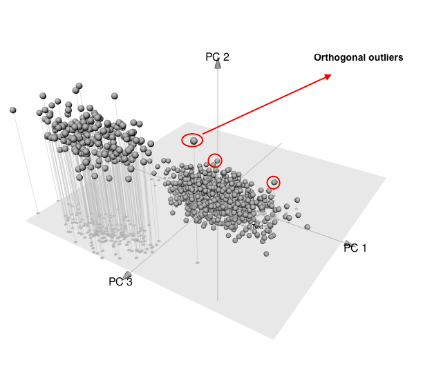
The three axes show the direction of principal components. Out of 1000 observations, only 20% of them are coming from different normal distribution. As it can be observed, these observations totally pulled the the first principle component into their direction. This could be of no desire since it does not reveal the property of the majority of data! Now, lets run another version of principle components which is assumed to be more robust to these outliers. 

Now, you can see how magically things have changed! In this graph, the first principle component is following the direction which majority of data varying in. This could help us to identify points which are potential outliers. In the following graphs, I highlighted the points which can be defined as some sort of outliers. This is possible through projecting the points into the principle component subspace. The two criteria of score distance and orthogonal distance could come in handy to diagnose these so called abnormal points. All these notions are shown in below graphs.

The points which have high orthogonal distance to PCA space and are remote from the center of typical data are called bad leverage points. As it has been observed these observations totally destroyed the usefulness of model. 

All in all, the outliers need to be identified and investigated in order to verify their existence in the model. 

 
require('simFrame')
require('mvtnorm')
require('rrcov')
require('pca3d')
sigma <- matrix(c(1, 0.5, 0.5,0.5,1, 0.5, 0.5, 0.5,1), 3, 3)
dc <- DataControl(size = 1000, distribution = rmvnorm, dots = list(sigma = sigma))
cc <- DCARContControl(epsilon = .2, distribution = rmvnorm, dots = list(mean = c(5, -5,5), sigma = sigma))
data<-generate(dc)
data_cont<-contaminate(data,cc)
pc<-prcomp(data_cont[,-4],center=TRUE,scale=TRUE)
Rob_pca<-PcaHubert(data_cont[,-4],scale=TRUE)
pca3d(Rob_pca@scores,show.shadows=TRUE,show.plane=TRUE)
pca3d(pc,show.shadows=TRUE,show.plane=TRUE)

Text Messages during Catastrophes without network, WiFi

Back in 2006, there was a fatal shooting in Montreal that made the news. It happened at Dawson College, which was one minute away on foot from another called Marianopolis College.

Since the two colleges were very close, and separated by a small forest, the police closed down the entrances of both, and of course, it was panic everywhere. Incidentally, parents and friends were hearing the news all over the city and beyond, and the cellular networks serving our area were literally swarmed by thousands of calls and messages. That was the very first time we experienced a communication cut-off in a crisis because of the network's overuse.

My example is not the best one in terms of catastrophes, but when you think of forever feared names like Sandy, Katrina, Ike and Arthur (sorry for people named those...), and of the hundreds of thousands of people desperately trying to get in touch with someone, anyone, and they couldn't because either the networks were way overused, or cellular towers were literally flying in the winds, then you know what situations I am referring to.

We're, as you know, extremely dependent on our smartphones today, so much so that if they stop working we find ourselves utterly lost and vulnerable. What are we supposed to do when we're let down by cellular towers!? Well, Daniela and Jorge Perdomo, a sister-brother team built a start-up in Brooklyn, N.Y. resolute on finding an answer to just that question. Together they launched a remote-control-sized device called the goTenna (see picture). What does it do?

Simply put, it uses long-range radio signals to send and receive encrypted text messages without passing through cellular networks!

There's no power around, no cellular network and no WiFi. Whether you find yourself in the midst of a natural (or otherwise) catastrophe, or on the less gloomy side, you simply went on a hike with some friends or to a concert, and you have no reception to be able to communicate with someone else, as long as two people have the goTenna with them, they can keep in touch using radio signals! Ingenious isn't it? The device is battery-powered; it can last 30 hours of use, or 18 months in standby. At an altitude of 10 meters, it has a range of about 2 kilometers, and at 150 meters, around 40 kilometers. It connects to both iOS- and Android- operated devices through Bluetooth, and is small enough to fit in a purse, a backpack or a suitcase.

Although it's currently being reviewed by the U.S. telecom regulator (the FCC), it's already possible to pre-order it on the goTenna website (with the all-too-likeable motto: "No Service? - No Problem!") for $149 US per pair!

Interesting right? What are your thoughts? Full story here: GoTenna lets smartphones send  texts without cell service, WiFi - Technology & Science - CBC News

Performance of GPU vs CPU

Illustrating Three Approaches to GPU Computing: The Mandelbrot Set

As you may know (a few post earlier), our research lab has equipped by a GPU (Graphics Processing Unit) server, called Tesla k40, and today I did my first experiment to realize the computational power of this parallel hardware versus 5th Generation Intel® Core™ i7 Processor.

The following example, taken from Matlab, shows how fast GPU performance can speed up computing. Using Parallel Computing Toolbox™ this code is then adapted to make use of GPU hardware in three ways:

1. Using the existing algorithm but with GPU data as input 
2. Using arrayfun to perform the algorithm on each element independently 
3. Using the MATLAB/CUDA interface to run some existing CUDA/C++ code 

Setup

The values below specify a highly zoomed part of the Mandelbrot Set in the valley between the main cardioid and the p/q bulb to its left.

A 1000x1000 grid of real parts (X) and imaginary parts (Y) is created between these limits and the Mandelbrot algorithm is iterated at each grid location. For this particular location 500 iterations will be enough to fully render the image.

Below is an implementation of the Mandelbrot Set using standard MATLAB commands running on the CPU.

Using gpuArray

When MATLAB encounters data on the GPU, calculations with that data are performed on the GPU. The class gpuArray provides GPU versions of many functions that you can use to create data arrays, including the linspace, logspace, and meshgrid functions needed here. Similarly, the count array is initialized directly on the GPU using the functionones.

With these changes to the data initialization the calculations will now be performed on the GPU:

Element-wise Operation

Noting that the algorithm is operating equally on every element of the input, we can place the code in a helper function and call it using arrayfun. For GPU array inputs, the function used with arrayfun gets compiled into native GPU code. In this case we placed the loop in pctdemo_processMandelbrotElement.m:

Note that an early abort has been introduced because this function processes only a single element. For most views of the Mandelbrot Set a significant number of elements stop very early and this can save a lot of processing. The for loop has also been replaced by a while loop because they are usually more efficient. This function makes no mention of the GPU and uses no GPU-specific features - it is standard MATLAB code.

Using arrayfun means that instead of many thousands of calls to separate GPU-optimized operations (at least 6 per iteration), we make one call to a parallelized GPU operation that performs the whole calculation. This significantly reduces overhead.

Working with CUDA

In Experiments in MATLAB improved performance is achieved by converting the basic algorithm to a C-Mex function. If you are willing to do some work in C/C++, then you can use Parallel Computing Toolbox to call pre-written CUDA kernels using MATLAB data. You do this with the parallel.gpu.CUDAKernel feature.

A CUDA/C++ implementation of the element processing algorithm has been hand-written in pctdemo_processMandelbrotElement.cu. This must then be manually compiled using nVidia's NVCC compiler to produce the assembly-level pctdemo_processMandelbrotElement.ptx (.ptx stands for "Parallel Thread eXecution language").

The CUDA/C++ code is a little more involved than the MATLAB versions we have seen so far, due to the lack of complex numbers in C++. However, the essence of the algorithm is unchanged:

                         

Summary

This example has shown three ways in which a MATLAB algorithm can be adapted to make use of GPU hardware:

1. Convert the input data to be on the GPU using gpuArray, leaving the algorithm unchanged
2. Use arrayfun on a gpuArray input to perform the algorithm on each element of the input independently
3. Use parallel.gpu.CUDAKernel to run some existing CUDA/C++ code using MATLAB data

Code

 
maxIterations = 500;
gridSize = 1000;
xlim = [-0.748766713922161, -0.748766707771757];
ylim = [ 0.123640844894862,  0.123640851045266];
%%%%%%%%%%%%%%%%%%%%%%%%%%%%%%%%%%%%%%%%%%%%%%%%%%%%%%
t = tic();
x = linspace( xlim(1), xlim(2), gridSize );
y = linspace( ylim(1), ylim(2), gridSize );
[xGrid,yGrid] = meshgrid( x, y );
z0 = xGrid + 1i*yGrid;
count = ones( size(z0) );
% Calculate
z = z0;
for n = 0:maxIterations
    z = z.*z + z0;
    inside = abs( z )<=2;
    count = count + inside;
end
count = log( count );
% Show
figure
hold on
cpuTime = toc( t );
fig = gcf;
fig.Position = [200 200 600 600];
imagesc( x, y, count );
axis image
colormap( [jet();flipud( jet() );0 0 0] );
title( sprintf( '%1.2fsecs (without GPU)', cpuTime ) );
hold off
%%%%%%%%%%%%%%%%%%%%%%%%%%%%%%%%%%%%%%%%%%%%%%%%%%%%%%
% Setup
t = tic();
x = gpuArray.linspace( xlim(1), xlim(2), gridSize );
y = gpuArray.linspace( ylim(1), ylim(2), gridSize );
[xGrid,yGrid] = meshgrid( x, y );
z0 = complex( xGrid, yGrid );
count = ones( size(z0), 'gpuArray' );

% Calculate
z = z0;
for n = 0:maxIterations
    z = z.*z + z0;
    inside = abs( z )<=2;
    count = count + inside;
end
count = log( count );

% Show
figure
fig = gcf;
fig.Position = [200 200 600 600];
hold on
count = gather( count ); % Fetch the data back from the GPU
naiveGPUTime = toc( t );
imagesc( x, y, count )
axis image
colormap( [jet();flipud( jet() );0 0 0] );
title( sprintf( '%1.3fsecs (naive GPU) = %1.1fx faster', ...
    naiveGPUTime, cpuTime/naiveGPUTime ) )
hold off
%%%%%%%%%%%%%%%%%%%%%%%%%%%%%%%%%%%%%%%%%%%%%%%%%%%%%%
% function count = pctdemo_processMandelbrotElement(x0,y0,maxIterations)
% z0 = complex(x0,y0);
% z = z0;
% count = 1;
% while (count <= maxIterations) && (abs(z) <= 2)
%     count = count + 1;
%     z = z*z + z0;
% end
% count = log(count);

% Setup
t = tic();
x = gpuArray.linspace( xlim(1), xlim(2), gridSize );
y = gpuArray.linspace( ylim(1), ylim(2), gridSize );
[xGrid,yGrid] = meshgrid( x, y );

% Calculate
count = arrayfun( @pctdemo_processMandelbrotElement, ...
                  xGrid, yGrid, maxIterations );

% Show
figure
fig = gcf;
fig.Position = [200 200 600 600];
hold on
count = gather( count ); % Fetch the data back from the GPU
gpuArrayfunTime = toc( t );
imagesc( x, y, count )
axis image
colormap( [jet();flipud( jet() );0 0 0] );
title( sprintf( '%1.3fsecs (GPU arrayfun) = %1.1fx faster', ...
    gpuArrayfunTime, cpuTime/gpuArrayfunTime ) );
hold off
% Load the kernel
cudaFilename = 'pctdemo_processMandelbrotElement.cu';
ptxFilename = ['pctdemo_processMandelbrotElement.',parallel.gpu.ptxext];
kernel = parallel.gpu.CUDAKernel( ptxFilename, cudaFilename );

% Setup
t = tic();
x = gpuArray.linspace( xlim(1), xlim(2), gridSize );
y = gpuArray.linspace( ylim(1), ylim(2), gridSize );
[xGrid,yGrid] = meshgrid( x, y );

% Make sure we have sufficient blocks to cover all of the locations
numElements = numel( xGrid );
kernel.ThreadBlockSize = [kernel.MaxThreadsPerBlock,1,1];
kernel.GridSize = [ceil(numElements/kernel.MaxThreadsPerBlock),1];

% Call the kernel
count = zeros( size(xGrid), 'gpuArray' );
count = feval( kernel, count, xGrid, yGrid, maxIterations, numElements );

% Show
figure
fig = gcf;
fig.Position = [200 200 600 600];
hold on
count = gather( count ); % Fetch the data back from the GPU
gpuCUDAKernelTime = toc( t );
imagesc( x, y, count )
axis image
colormap( [jet();flipud( jet() );0 0 0] );
title( sprintf( '%1.3fsecs (GPU CUDAKernel) = %1.1fx faster', ...
    gpuCUDAKernelTime, cpuTime/gpuCUDAKernelTime ) );
hold off

Optimization models for wood procurement activities

In forest industry, procurement activities planning is a complex task. It requires taking into account a lot of information such as forest inventories, final products demand, seasonality in forest sectors and production capacity. This information should be provided by different stakeholders in the supply chain such as mill managers, forest engineers, sales managers, etc. The collaboration between these stakeholders is necessary to exchange information and support the planning task.

Several researches have been done in order to support forestry companies in improving their planning process and thus making better decisions. For this purpose, some authors adopted an operational research approach. Previous work showed that optimization models can be integrated into forest manufacturing processes and that they help planning forestry operations efficiently and easily. In fact, they reduce planning time as most of them (models designed to plan transport, harvesting, etc.) take only a few minutes to find the optimal solution. Furthermore, it has been proved that they increase profit by more than 5%.
However, despite their advantages, optimization models are rarely implemented in the forest industry. They do not meet the companies needs. Indeed, planning is still done manually, by a trial/error approach. Engineers rely on their knowledge, experiences and intuitions to plan different activities (harvesting, processing in mills, sales, etc.).
What could be the reasons limiting the adoption of these models by forestry companies?

Of programming for machine learning, speed and Julia

Machine learning is really about exploring models, moving around and modifying code. Indeed, in machine learning, the level of abstraction developers expect is quite higher than what c/c++ would easily allow. When you are in exploration for new models and new solutions, you want to be able to, from the start, write code at a level of abstraction as close as possible to straight math equations. This explains the popularity of languages like R and Matlab, as these languages allow the user to write code and think in equations and tensors instead of thinking in containers, types and references.

The problem with these scripting languages is that they are extremely slow, as shown in the following graph, taken on www.julialang.org/ (the unit (value of 1) of this table is the value of the C execution time). While these numbers truly only show part of the picture, I think that if you look around on the net you will quickly find that none of these numbers are really controversial.

Recently, Python has gained huge popularity in the world of machine learning, as Python is indeed great fairly high level programming language with a huge community, and because NumPy provides awesome Matlab-like tensor manipulation with typed, fast operations implemented in native languages (C/C++/Fortran). Python, however, has some really big limitations. Indeed, the main implementation of the language only uses a straight bytecode interpreter, and offers no way to restrict dynamic typing to allow for optimization. As such, it is pretty slow (although still being much faster than R and Matlab). Its reliance on old, non-thread-safe C code forced the developers of CPython to implement what is known as the Global Interpreter Lock. Basically, it means that a single Python interpreter process can only have one thread executing bytecode at the time. What this means is that any non IO based shared memory multithreading (not to be confused multiprocessing) is impossible, greatly limiting the options for parallelism in Python.

Enter Julia. Julia is a JIT (Just In Time) compiled language, meaning that instead of simply interpreting bytecode, the subroutines are compiled to native language slightly in advance. This allows for the following executions of a functions or a loop to be much quicker than they would be if they were interpreted at each pass. The fact that the code is actually compiled instead of just being interpreted also allows fir static analysis and optimisation to be made on the code, for exemple removing code with no visible end effects (dead code), propagating constants, etc. Julia also has optional static typing, allowing for even greater static analysis and optimization.
Shared memory parallelism is still being developed for Julia. There is currently a working implementation of a thread safe demonstration version of Julia for Linux, but code still needs to be produced in order for Julia to support shared memory parallelism in other mainstream platforms.

An other extremely interesting feature Julia has is that it was built to be incredibly easy to interface with C/C++ and with Python. Note here that when I say incredibly easy, it's no exaggeration. Some examples of code integration can be observed here for C, and here for Python.

Julia also fully supports IPython style online notebooks, like this :

It also has a beautiful plotting library in Gadfly, aside from being able to use Matplotlib really easily:

All in all, even though Julia is still a bit too young to be fully considered for production code, it is an extremely promissing project that I would watch really closely.

We teach to machines

The science of data is a hot topic nowadays, everybody knows!

The amount of measurements that our smart phone stores or has access to, can be compared with all of the science for many centuries. This allows us to start analysing people's behaviour and understand how they behave and why. Your mobile phone knows your secrets much more than anybody else, you may lie to somebody, but it is difficult to lie to your mobile phone. 

Now we need to innovate some robots to tell us what does this massive data mean! But why robots? because we cannot do it ourselves.

Analysis of such a massive data requires a lot of mathematical operations that a human being during his life cannot do, even a small portion of it (even using a calculator).

We make some machines and teach them to learn and then analyse data. We require a bunch of machines to do the analysis more efficiently, because your data keep growing as your life goes on. We (humans) learn collectively by dividing the task beween us and aggregating the final result. The new generation of computing machines such as the GPU and the CPU servers benefit this model. They  implement several tasks independently, and aggregate the final result eventually.

Our Tesla K40 is installed today at Poly, try some parallel computing tasks there.

Probability and non-measurablity

In the measure-theoretic axioms of probability theory, probability is defined as a measure on a set of measurable subsets (called a \(\sigma\)-algebra) of the sample space. Although, in practice we (especially if we are not interested in the mathematical foundations of probability theory) do not usually care about this and intuitively expect any subset of the sample space to be measurable (i.e., to be a random event) and be capable to be assigned a non-negative value as the probability of that event to happen. In fact, this is our intuition that suggests any subset of the sample space being a random event. Until the other day when we were discussing this with Vahid, I never had thought why we do not simply replace the notion of \(\sigma\)-algebra in the definition of the probability space by the power set of the sample space. I was unconsciously convinced that we define the probability measure on a \(\sigma\)-algebra of subsets just because generally we do so in measure theory, i.e., if a collection of sets is a \(\sigma\)-algebra then of course we can define a measure on it. And moreover, I was convinced that defining the probability on a \(\sigma\)-algebra, instead of just the power set, which is by definition the biggest \(\sigma\)-algebra, is only a more formal way of defining the probability as a measure. The problem is that, in particular cases, not all of the subsets of a sample space can be measured. The Banach-Tarski theorem gives an example of such a case. According to Banach-Tarski theorem, given a \(3\)-dimensional solid ball one can decompose it into a finite number of pairwise disjoint subsets and put them back together in a different way to yield a new ball whose radius is two times bigger than the original one!

The process of reassembly involves only rotations and translations, without any stretching, bending, or adding new points. But what is the connection between this counter-intuitive result and measurability of subsets of the sample space? Let \(S\) be a \(3\)-dimensional ball whose radius is greater than \(0\) and let \(\mu(A)\) denote the volume of \(A\), where \(A\) is a subset of \(S\). Suppose we split \(S\) into disjoint subsets \(S_{1},S_{2},\dots S_{n};\, n\in\mathbb{N}\) and reassemble them, in the aforementioned manner, to get the new ball \(S^{\prime}\) with \(\mu(S^{\prime})=2\mu(S)\). The last equality implies that \[ \mu(S_{1}\cup S_{2}\cup\dots\cup S_{n})=2\mu(S_{1}\cup S_{2}\cup\dots\cup S_{n})\Rightarrow \] \[ \mu(S_{1})+\mu(S_{2})+\dots\mu(S_{n})=2[\mu(S_{1})+\mu(S_{2})+\dots\mu(S_{n})] \] Since not all of \(S_{1},S_{2},\dots,S_{n}\) are empty, one of the possible scenarios is that there exist subsets which are not measurable! As you see the possibility of existence of non-measurable sets is surely a "good" reason to restrict ourselves to \(\sigma\)-algebras for defining the probability measure, as we definitely do not want our definitions to be "formally" wrong. Apparently, doing this we are exonerated from the allegation of "being mathematically wrong". However, one can still question the validity of the Banach-Tarski theorem in the "real" world. Even more generally, does really the "mathematical world" always fit the actual world?!